S P L A T I F Y

Paper → Code → Discover

A Claude agent reads a 3DGS paper end-to-end and writes the implementation. Then 8 specialized agents compete across generations to discover a novel method that beats the baseline — live.

GAUSSIAN SPLATTING · READ · REASON · WRITE · RENDER · DISCOVER
arxiv:2308.04079› 3D Gaussian Splatting› parse
orchestrator
tokens 0
model claude-opus-4.7
00:00.0
parse
›
read
›
citations
›
plan
›
code
›
render
›
fix
USER
arena
›
evolve
›
champion
›
render
P
gaussian_splatting_2308.04079.pdf
PDF · arxiv

3D Gaussian Splatting for Real-Time Radiance Field Rendering

Bernhard Kerbl · Georgios Kopanas · Thomas Leimkühler · George Drettakis
ACM SIGGRAPH 2023 · Inria & MPII
Abstract. Radiance field methods have achieved photo-realistic synthesis of scenes captured with multiple photos. We introduce three key elements: (1) starting from sparse SfM points, we represent the scene with 3D anisotropic Gaussians; (2) we interleave optimization with adaptive density control; (3) we develop a fast visibility-aware, tile-based rasterizer. Real-time rendering at state-of-the-art quality.
1Introduction

Radiance field methods, starting with NeRF, have achieved high-quality novel-view synthesis from a set of photos. However, volumetric MLPs are slow to train and render. We propose an explicit representation: a set of 3D Gaussians that can be projected and composited via a tile-based GPU rasterizer.

33D Gaussian Representation

We represent the scene as a set of N 3D Gaussians, each with a mean μ, a covariance matrix Σ, an opacity α, and spherical-harmonic (SH) color coefficients for view-dependent appearance:

G(x) = exp(−½(x−μ)ᵀ Σ⁻¹ (x−μ)) (1)

For optimization stability Σ is parameterized via a rotation R (quaternion) and a diagonal scale S:

Σ = R S Sᵀ Rᵀ (2)
3.1Differentiable Tile Rasterization

We project each 3D Gaussian to 2D, sort by depth inside 16×16 tiles, and composite front-to-back using α-blending identical to NeRF's volume rendering:

C(p) = Σᵢ αᵢ Tᵢ cᵢ(d),    Tᵢ = Πⱼ<ᵢ (1 − αⱼ) (3)

The rasterizer is fully differentiable and written in CUDA; gradients flow through the α-blending to position, scale, rotation, opacity, and SH coefficients.

3.2Optimization

We supervise rendered images with the photometric L1 loss combined with a D-SSIM term:

L = (1 − λ) L₁ + λ LD-SSIM,  λ = 0.2 (4)

We use Adam with exponentially-decaying learning rates on positions (1.6×10⁻⁴ → 1.6×10⁻⁶). Opacities, scales, rotations and SH coefficients have separate learning rates. Training runs 30,000 iterations.

3.3Adaptive Density Control

Every 100 iterations, we densify and prune Gaussians based on the magnitude of the view-space position gradient ∇pL:

  • Clone: small Gaussians (‖s‖ < τs) with high gradient → duplicate and nudge along gradient.
  • Split: large Gaussians with high gradient → split into two smaller Gaussians with s ← s/1.6.
  • Prune: Gaussians with opacity α < εα or world-space scale > 10% of scene extent are removed.
figure 4 · densification
4Implementation & Results

We implement the rasterizer in CUDA and the optimizer in PyTorch. MipNeRF360 outdoor scenes train to 27+ PSNR in ~30 minutes on an A6000 and render at 130 FPS at 1080p.

Hyperparameters: SH degree 3, densification from step 500 to 15000, opacity reset every 3000, gradient threshold 2×10⁻⁴, λssim = 0.2.
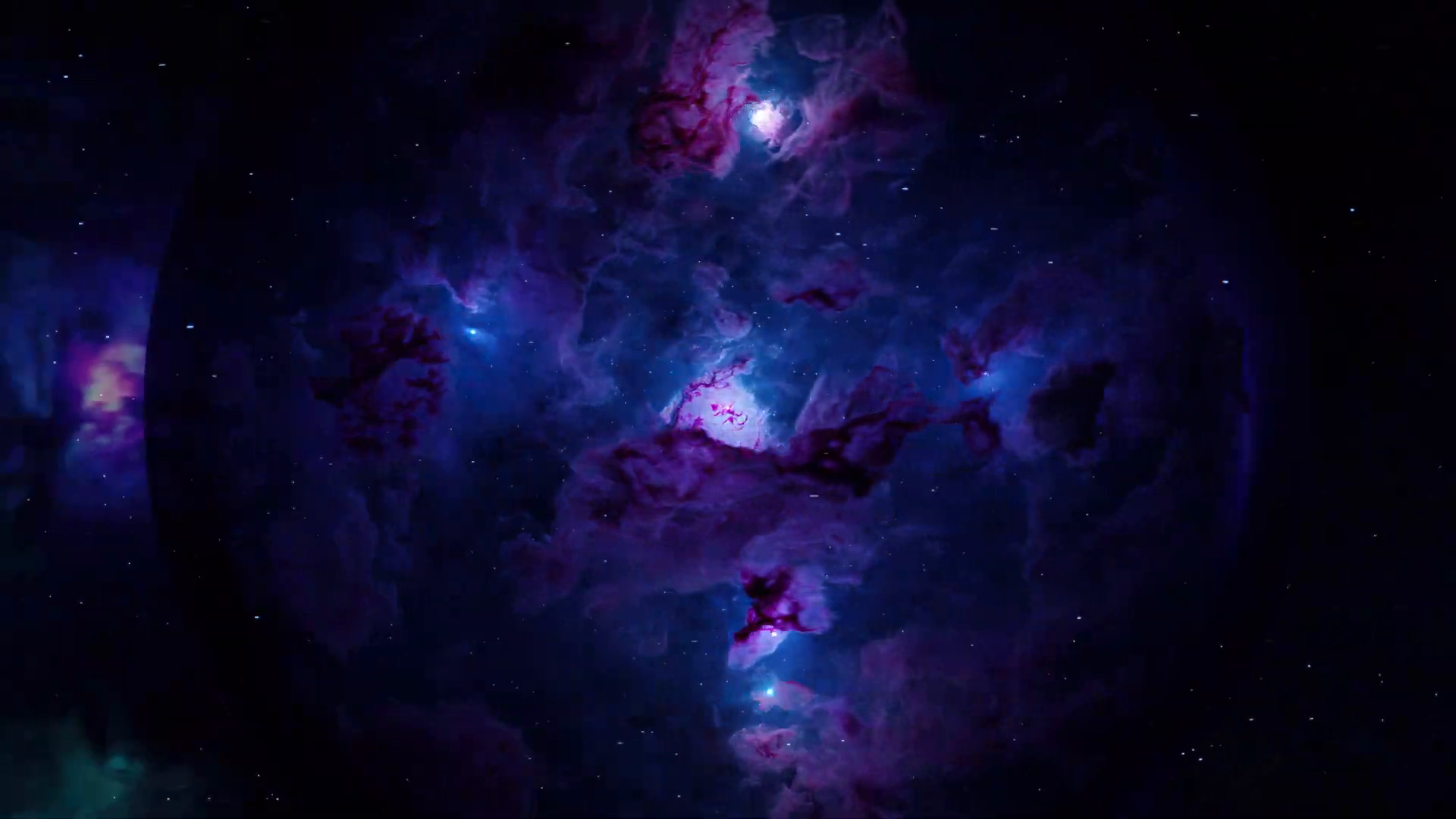
figure 7 · comparisons
References
[1] Mildenhall et al. NeRF: Representing Scenes as Neural Radiance Fields. ECCV 2020.
[2] Mueller et al. Instant-NGP: Instant neural graphics primitives. SIGGRAPH 2022.
[3] Barron et al. Mip-NeRF 360: Unbounded anti-aliased neural radiance fields. CVPR 2022.
[4] Zwicker et al. EWA Splatting. IEEE TVCG 2002.
1 / 14
A
Agent · reasoning
LIVE
Booting orchestrator
claude-opus-4.7 · temperature 0.2
extracted concepts
</>
gs_template — generated
model.py
📄model.py
📄losses.py
📄rendering.py
📄configs.py
generating model.py
lines 0 • PYTHON • UTF-8
DrJohnson rendering 4 preview frames…
iter 3000 · PSNR 22.4
view 0
view 0 · front21.8
view 1
view 1 · side22.6
view 2
view 2 · back22.1
view 3
view 3 · wide23.0
! floaters in low-density regions (visible on view 0, 2)
! over-opaque Gaussians on specular highlights (view 1)
! opacity reset interval too aggressive — losing detail at 3000
✓
Paper implemented · baseline rendered
8 files · 1 fix iter · 27.1 PSNR · 0 errors
PSNR 27.1 ✓
S
you · just now
splatify orchestrator
GEN 1 R1 · 2k iters · 8 → 4
🏟️ Knowledge Discovery Arena 8 island agents · parallel evolutionary tournament
Baseline: 28.30 dB · Best: — dB
📊 Live PSNR Race step 0 / 2000
📚 Knowledge Ledger COMPOUNDS ACROSS GENS
★ NOVEL METHOD DISCOVERED ★
NebulaGS
Physics-Informed Gaussian Splatting for Volumetric Emission
PSNR
31.72
Δ Baseline
+3.42
Generations
3
Techniques emerged through cross-generation knowledge transfer:
L1
Linear warmup on physics losses (0 → 0.008) over first 3k steps — gentle priors, not hard constraints
L2
Opacity ceiling at 0.95 instead of pushing to 0.5 — preserves emission semantics
L3
Per-Gaussian emission_rgb parameter (synthesized from Gen 1 + 2 winners)
L4
Multi-scale L1 reconstruction loss (λ=0.5) — cooperates with main L1, stable
nebulags · live · 30fps
NebulaGS · garden · 31.72 dB
Rendering NebulaGS output…

🏆 Discovery Complete

31.72 dB
Baseline: 28.30 dB · +3.42 dB ✓ BEAT
DiscoveredNebulaGS
Datasetvolumetric nebula
Islands Trained24 (8 × 3 gens)
Knowledge Entries17
Debug Fixes3 cycles
Tokens2,987,421
Cost$12.84
Duration47m 12s

📦 GENERATED PACKAGE9 files